auto_explain vs pg_stat_statements in production

pg_stat_statements and auto_explain are the two diagnostic extensions every production Postgres instance should run. They are regularly framed as competitors. They are not. pg_stat_statements aggregates cost across calls and answers "what is expensive across the workload." auto_explain captures the plan for slow executions and answers "why was a specific run expensive." A correct regression detector reads both. Most dedicated monitoring tools read one and compensate with heuristics for the other. This post is a technical reference for when each one lies, and the specific queries to run when you need to cross-check. For the triage-to-fix workflow these signals feed on a managed project, see the Supabase query performance guide.

TL;DR. Use pg_stat_statements to rank queries by aggregate cost and detect regressions in total time or I/O. Use auto_explain to see the plan that produced a specific slow execution. Join the two through the queryid and the normalized query text. Add pg_stat_kcache for OS-level I/O and CPU attribution per query. Each signal has a specific failure mode: pg_stat_statements cannot distinguish a plan change from a data-growth regression; auto_explain only sees the plan that actually ran, not the plans that did not.

What each one actually sees

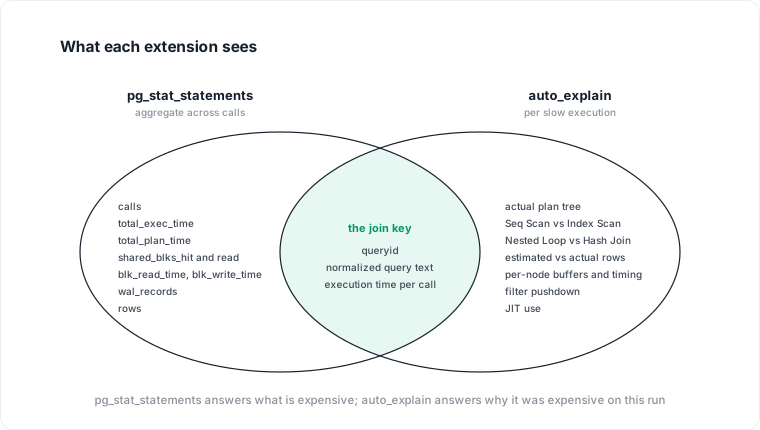
The left-only and right-only regions are where each extension uniquely reports. The overlap is the join key.

pg_stat_statements: aggregate cost per normalized query

The Postgres documentation is explicit about what pg_stat_statements does: it "tracks planning and execution statistics of SQL statements." One row per distinct combination of database ID, user ID, query ID, and (since Postgres 14) whether the statement was top-level. The metrics are cumulative totals and summary statistics: total_exec_time, min_exec_time, max_exec_time, mean_exec_time, stddev_exec_time; similarly for total_plan_time in Postgres 13+. Block counts for shared, local, and temp buffers (hits, reads, dirtied, written). I/O timing, WAL records, JIT counters, parallel worker counts, and rows. It is a long list of scalar aggregates per normalized query.

The view does not store the execution plan. The query text is the normalized form, with literals replaced by parameter placeholders. The resolution is one entry per distinct query shape, not one per execution.

auto_explain: full plan per slow execution

The auto_explain module logs execution plans automatically when they exceed a duration threshold. The key parameter is auto_explain.log_min_duration, set in milliseconds. Everything longer than that gets its plan logged. The logged plan is whatever EXPLAIN would have produced, optionally with ANALYZE, BUFFERS, and TIMING details.

The documentation carries a specific performance warning: log_timing "causes per-plan-node timing to occur for all statements executed, whether or not they run long enough to actually get logged. This can have an extremely negative impact on performance." In production, log_analyze = on, log_buffers = on, log_timing = off is the standard combination. The plan shape and buffer counts are retained; per-node timing is not.

auto_explain produces one log entry per slow execution. It does not aggregate and it does not store historical trends. Its output is a stream of plans indexed by time, written to the Postgres log.

The failure modes

Each extension lies in a specific way that the other one can catch, if you are reading both.

Where pg_stat_statements cannot see

A query's mean_exec_time doubles overnight. The call count is stable. The row count is stable. The buffer reads are up. From pg_stat_statements alone, this could be three different regressions: the plan changed (e.g., an index got dropped), the data grew (more rows scanned per call), or I/O got slower (the underlying storage is degraded). The view exposes the symptom. It does not distinguish the three causes.

The distinction matters because the fixes differ. A plan change is fixed by restoring the index or forcing a plan. Data growth is fixed by rewriting the query, adding an index, or partitioning. Slower I/O is a capacity issue. pg_stat_statements does not tell you which one.

Where auto_explain cannot see

An auto_explain entry is one run. If the run you captured ran a Seq Scan on a 12M-row table, you know the plan was bad for that run. You do not know whether every other run of the same query uses the same bad plan or whether this one was an outlier because the planner chose differently under load. A single captured plan cannot report distributional information.

And auto_explain only captures runs that exceeded the duration threshold. Shorter runs of the same normalized query, which might be hitting a different plan or a warmer cache, are invisible. If the threshold is 1000 ms and the problematic plan sometimes takes 900 ms, the diagnostic never fires.

The two blind spots meet in the N+1 cascade. Every individual execution is fast, so auto_explain never fires on any of them, and ranking pg_stat_statements by mean_exec_time buries the pattern near the bottom of the list. Reading a cascade out of pg_stat_statements means sorting on calls instead, and comparing that count across a deploy boundary rather than at one point in time.

Reading them together

The two views join naturally. Both expose queryid (a stable hash of the normalized query). pg_stat_statements stores it as a column. auto_explain logs it alongside the plan when compute_query_id is enabled at the server level. The join across the two signals is the combination a regression detector needs.

The practical query to rank regressions from pg_stat_statements:

-- Top 20 candidates for a regression check, ranked by
-- total time change against a prior snapshot.
WITH now_s AS (
  SELECT queryid, query, calls, total_exec_time
  FROM   pg_stat_statements
),
prior_s AS (
  SELECT queryid, calls AS prior_calls, total_exec_time AS prior_total
  FROM   pg_stat_statements_history  -- your rolled-up snapshot table
  WHERE  captured_at = (SELECT max(captured_at)
                        FROM   pg_stat_statements_history
                        WHERE  captured_at < now())
)
SELECT n.queryid,
       n.query,
       (n.total_exec_time - p.prior_total) AS delta_exec_ms,
       (n.total_exec_time::numeric / NULLIF(n.calls, 0))
       - (p.prior_total::numeric / NULLIF(p.prior_calls, 0)) AS delta_mean_ms
FROM   now_s n
JOIN   prior_s p USING (queryid)
ORDER  BY delta_exec_ms DESC
LIMIT  20;

That ranks the queries where total time has grown most since the last snapshot. For each candidate, the next step is to find the plan. If auto_explain is logging with compute_query_id enabled, the log contains plan entries tagged with the same queryid. A grep against the Postgres log for the offending queryid surfaces the plan of any slow execution captured since the threshold was set. The delta from the plan shape on the old side to the new side is the attribution.

The combined reading: pg_stat_statements says "query X got 3x slower in total time." auto_explain says "here is the plan that ran this morning." The comparison against the historical plan (if any captured) or the prior-known-good plan for the same queryid says "the planner switched from Index Scan on idx_orders_user to Seq Scan on orders." Three separate statements, each from a different source, that together name the regression.

Where the add-on extensions help

Two companion extensions are worth running alongside.

pg_stat_kcache

pg_stat_kcache, from the PoWA team, gathers OS-level statistics per query: real disk reads and writes (below the OS page cache), user and system CPU time, context switches. It requires pg_stat_statements to be loaded alongside it; the two share the queryid dimension.

The reason to run it: the shared_blks_read column in pg_stat_statements counts blocks read by Postgres, not blocks that actually hit the disk. A query that reads 1M blocks from Postgres's shared buffer cache but whose working set is entirely in the OS page cache has very different physical cost than one whose reads go to disk. pg_stat_kcache surfaces this distinction via reads and writes columns measured in bytes at the getrusage layer.

Combined with pg_stat_statements, this answers "is this query I/O-bound at the OS level or CPU-bound," which the standard view cannot answer directly. For the regression case, it distinguishes a plan change that added CPU work (e.g., a Hash Join over a larger input) from one that added I/O work (e.g., a Seq Scan on a previously-indexed table).

pg_stat_plans

pg_stat_plans aggregates statistics per plan, not per normalized query: the cost of each distinct plan a query has been observed to use. This is specifically the distribution information that auto_explain cannot give you, because auto_explain only logs the plan of a single slow run, not the set of plans seen across all runs. The original 2ndQuadrant extension of that name is unmaintained; pganalyze shipped a fresh implementation in 2025 that tracks per-plan call counts, execution times, and EXPLAIN texts on Postgres 16 and newer.

The extension is less widely deployed than pg_stat_statements and auto_explain. On managed Postgres services it is often not available. When it is, it closes the one specific gap the base pair leaves: "is this query sometimes running on a different plan, and which plan produces the regression." Without it, the same question is answered by correlating pg_stat_statements time variance against auto_explain plan samples, which is approximate.

A reading of the two signals against one another

Practical setup recipe

The minimal configuration for a production Postgres instance that wants both signals.

# postgresql.conf

# load both extensions
shared_preload_libraries = 'pg_stat_statements,auto_explain'

# enable query IDs so the two views join cleanly
compute_query_id = on

# pg_stat_statements
pg_stat_statements.max = 10000
pg_stat_statements.track = all
pg_stat_statements.track_planning = on  # Postgres 13+

# auto_explain: capture plans for any execution over 1s
auto_explain.log_min_duration = 1000
auto_explain.log_analyze = on
auto_explain.log_buffers = on
auto_explain.log_timing = off   # per-node timing is expensive
auto_explain.log_verbose = off
auto_explain.log_nested_statements = off

# write logs somewhere you will actually read them
log_directory = 'pg_log'
log_rotation_size = 1GB

The single most important line is compute_query_id = on. Without it, the two extensions exist but do not share a join key. Every query in the log has to be identified by text, which is brittle across parameterized queries and error-prone at scale.

What this does not cover

Reading both signals tells you what is slow and what plan it is running. It does not tell you which commit caused the plan to change. That is the attribution problem covered in detail in the earlier post on the attribution gap. The two extensions are inputs to an attribution pipeline; they are not the attribution pipeline themselves. A layer that reads both and resolves them against what the schema actually means is what turns raw diagnostics into context a team or an agent can act on. That layer is what Datapace is building.

Closing note

The instinct to pick one of these extensions and evangelize it is worth resisting. They answer different questions. A team that runs only pg_stat_statements can rank regressions but cannot name their cause. A team that runs only auto_explain can see a plan but has no idea whether it matters. A team that runs both, with compute_query_id enabled and pg_stat_kcache optional, has the raw signal a regression detector needs. The detector on top of that raw signal is a separate layer; what this post covers is the foundation both the DIY and the productized versions depend on.

Datapace is building the context layer between your databases and your AI: what the schema means, the operational reality around it (cost, performance, usage, lineage), and a policy gate over what AI may do, served to agents over MCP. On Postgres, these two extensions feed the operational half of that picture. Turning both signals into machine-usable context an agent can trust is what we are building on top. If you would like to compare notes, book a call with us.

Sources

1. PostgreSQL documentation, pg_stat_statements (current version).
2. PostgreSQL documentation, auto_explain (current version).
3. PoWA team, pg_stat_kcache GitHub repository.
4. EDB / 2ndQuadrant, pg_stat_plans historical repository.
5. pganalyze, pg_stat_plans GitHub repository (current implementation, Postgres 16+).
6. M. Ma, Z. Yin, S. Zhang et al., "Diagnosing Root Causes of Intermittent Slow Queries in Cloud Databases" (iSQUAD), PVLDB 13(8), 2020.
7. Datapace blog, "The attribution gap: why DB research can't name the commit".
8. Datapace blog, "Why generic time-series anomaly detection fails on Postgres".