Supabase query performance: find, read, and fix slow queries

TL;DR. Supabase enables pg_stat_statements on every project, so slow-query triage starts with two SQL queries: rank by total_exec_time for aggregate cost, rank by mean_exec_time for per-call pain. Diagnose the offenders with EXPLAIN (ANALYZE, BUFFERS), where shared read counts the disk I/O that actually costs money. The most common finding is a sequential scan on a growing hot table, which drives both the latency and the compute upgrade that quietly doubles the bill. One CREATE INDEX CONCURRENTLY usually fixes both.

A slow Supabase project is almost never slow everywhere. It is slow in two or three query shapes, and the whole diagnostic job is identifying which ones, reading why they are slow, and fixing them without taking the database down. Postgres ships everything required: pg_stat_statements ranks the workload, EXPLAIN (ANALYZE, BUFFERS) explains one query, and CREATE INDEX CONCURRENTLY applies the most common fix without blocking writes. This guide walks that pipeline end to end, with real output. On the example workload below, one missing index is the difference between 2,847 ms and 0.82 ms per call.

The order matters. Running EXPLAIN ANALYZE on queries your team suspects are slow means diagnosing the wrong set. The right set is whatever pg_stat_statements says is expensive in aggregate across everything your application actually runs, and that set rarely overlaps cleanly with engineering intuition. Triage with statistics first, then diagnose.

Find the culprits with pg_stat_statements

pg_stat_statements is a standard extension, distributed with Postgres, that keeps a running tally for every normalized query executed on the server. Normalization strips literals: SELECT * FROM users WHERE id = 123 and SELECT * FROM users WHERE id = 456 are the same statement, counted together. For each distinct statement it records calls, total_exec_time, the distribution of execution time (mean_exec_time, min, max, stddev), rows returned, and buffer cache hits versus disk reads.

On Supabase it is enabled by default on every project. Nothing to install. Verify with SELECT * FROM pg_available_extensions WHERE name = 'pg_stat_statements';. On self-hosted Postgres, add it to shared_preload_libraries, restart, and run CREATE EXTENSION pg_stat_statements; in each database you want to measure. RDS, Cloud SQL, and Neon all support it too, usually behind a one-click toggle.

There are many ways to slice the view. Two cover 90 percent of real-world use.

The total-pain query:

SELECT
  substring(query, 1, 100) AS query,
  calls,
  round(total_exec_time::numeric, 1) AS total_ms,
  round(mean_exec_time::numeric, 2) AS mean_ms,
  rows
FROM pg_stat_statements
ORDER BY total_exec_time DESC
LIMIT 20;

The frustration-finder query:

SELECT
  substring(query, 1, 100) AS query,
  calls,
  round(mean_exec_time::numeric, 2) AS mean_ms,
  round(stddev_exec_time::numeric, 2) AS stddev_ms,
  rows / GREATEST(calls, 1) AS mean_rows
FROM pg_stat_statements
WHERE calls > 100
ORDER BY mean_exec_time DESC
LIMIT 20;

Filtering on calls > 100 removes one-off queries that ran once during a migration and took a second. The useful result is a query that runs many times and still averages badly per call: the signature of a missing index, a bad plan, or a lock wait.

Reading the output

A typical result looks like this (truncated):

               query                |  calls  | total_ms  | mean_ms |  rows
------------------------------------+---------+-----------+---------+--------
 SELECT ... FROM orders JOIN cust.. | 184,382 | 1,284,110 |    6.96 |    1.0
 SELECT * FROM pg_stat_statements   |     218 |   172,040 |  789.17 |  215.0
 UPDATE sessions SET last_seen_at.. |  92,110 |   112,220 |    1.22 |    1.0
 SELECT * FROM products WHERE sto.. |   1,204 |    98,400 |   81.72 |  502.0
 SELECT name FROM users WHERE id.. |2,147,883 |    66,040 |    0.03 |    1.0

Row 1 is the biggest total cost, a join running hundreds of thousands of times a day at 7 ms per call. Fine per call. If a fix is needed, it is caching or calling the endpoint less, and neither is a database change.

Row 2 is the extension itself. Your diagnostic queries show up in their own output. Ignore.

Row 4 is an 82 ms query running 1,204 times. Small total, bad mean. This is the row that deserves EXPLAIN (ANALYZE, BUFFERS), because 82 ms for 500 rows usually means a missing index or a filter that defeats the indexes that exist.

Row 5 is the N+1 signature. Two million calls at 0.03 ms each, individually invisible, collectively the fifth-largest total in the table. The fix is a join in the calling code, and reading the cascade out of the plan is its own skill: the signal is calls, never mean_ms.

One more useful trick: SELECT pg_stat_statements_reset(); zeroes the counters. Reset at deploy time, let an hour of production traffic run, and the view shows exactly what the new version of the application does. Without a before-and-after boundary, pg_stat_statements is a snapshot of the present, and a regression that shipped last week reads as normal.

Read the plan with EXPLAIN (ANALYZE, BUFFERS)

Once triage names a query, Postgres offers three levels of information about it. They are concentric: each adds to the previous without replacing it.

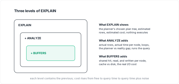
Each ring contains the previous one. BUFFERS does not replace ANALYZE. ANALYZE does not replace EXPLAIN.

Plain EXPLAIN asks the planner for its plan without executing anything: useful for a write you do not want to run, and for checking whether a query will hit an index at all. The cost figures it prints are estimates in an arbitrary unit calibrated to sequential page reads, comparable only between candidate plans for the same query. If the row estimate is wildly off from what you know the table holds, the statistics are stale and ANALYZE <table> (the maintenance command) will change the plan.

Adding ANALYZE runs the query for real and prints actual row counts and actual time per plan node next to the estimates:

EXPLAIN ANALYZE SELECT * FROM orders WHERE total > 500;

                          QUERY PLAN
----------------------------------------------------------------------
 Seq Scan on orders
   Filter: (total > 500)
   Rows Removed by Filter: 99,400
   (cost=0.00..2,451.00 rows=600 width=132)
   (actual time=0.012..18.450 rows=600 loops=1)
 Planning Time: 0.118 ms
 Execution Time: 18.502 ms

Postgres read every row in orders, kept the 600 that matched, discarded 99,400. After CREATE INDEX on total, the node changes to Index Scan and execution time drops from 18 ms to 0.7 ms: same data, same result, 26x faster. Three signals to read on every EXPLAIN ANALYZE: estimated versus actual rows (off by more than 10x means the planner is flying blind), where the time concentrates node by node, and any Sort, Hash, or Nested Loop sitting on a large input.

The BUFFERS level

Execution time is a symptom. The cause is usually I/O, and BUFFERS is the only option that shows it. Postgres stores tables and indexes in 8 KB pages. A buffer hit means the page was in shared memory; a buffer read means it came from disk, which is orders of magnitude slower on any real system. Since PostgreSQL 18, EXPLAIN ANALYZE includes buffer counts by default; on the version Supabase currently runs, ask for them explicitly with EXPLAIN (ANALYZE, BUFFERS).

EXPLAIN (ANALYZE, BUFFERS) SELECT * FROM orders WHERE total > 500;

 Index Scan using orders_total_idx on orders
   Index Cond: (total > 500)
   (actual time=0.047..0.612 rows=600 loops=1)
   Buffers: shared hit=72
 Execution Time: 0.698 ms

Seventy-two buffers hit, zero reads, so the whole query worked from cache. The same query run cold, right after a restart, reports shared hit=4 read=68 and takes 8.2 ms: same plan, same rows, twelve times slower purely because the pages came from disk. Without BUFFERS, two runs of the same query look unexplainedly different.

Four counters to know: shared hit (pages already in memory, cheap), shared read (pages from disk, expensive), shared dirtied (pages the query modified), shared written (pages flushed during the query). A query reporting shared read=40,000 pulled 320 MB off disk, and disk I/O is the cost that scales on a cloud database. For team review of a hot plan, EXPLAIN (ANALYZE, BUFFERS, FORMAT JSON) produces output that tools can diff, and explain.depesz.com renders any text-format plan as a highlighted tree.

What a sequential scan actually costs

The pattern the pipeline above finds most often is a Seq Scan on a hot, growing table. Sequential scans are the correct plan on small tables, where the whole table fits in a handful of pages. They become a problem when a hot read path runs one against a table that keeps growing, because the cost of the scan grows with the table while the query stays byte-for-byte identical in the codebase.

Concrete. Consider a sessions table with 50 million rows at 240 bytes per row (12 GB), and SELECT * FROM sessions WHERE user_id = $1 running five thousand times per minute:

EXPLAIN (ANALYZE, BUFFERS) SELECT * FROM sessions WHERE user_id = 12345;

 Seq Scan on sessions
   Filter: (user_id = 12345)
   Rows Removed by Filter: 49,999,988
   Buffers: shared hit=1,024 read=1,570,432
   (actual time=2,104.220..2,847.190 rows=12 loops=1)
 Execution Time: 2,847.412 ms

Every call reads 12 GB of pages, most from disk, in about three seconds. Five thousand calls per minute at three seconds each is 250 minutes of database CPU per wall-clock minute, which on any realistic instance means saturation. After CREATE INDEX CONCURRENTLY ON sessions (user_id); the same query reports Buffers: shared hit=16 read=2 and finishes in 0.82 ms. Buffer reads drop from 1.5 million to 18. Execution time drops 3,472x.

The billing consequence follows directly, because managed Postgres pricing is dominated by compute and I/O. When a scan like this pushes CPU to 80 percent at peak, the rational response under pressure is a larger instance, and that migration is usually permanent: nobody scales back down after the scan is quietly fixed a month later, because nobody connects the two events. The extra instance size is then paid every month, indefinitely, for a problem that was one index away from not existing. The performance problem and the cost problem are the same sequential scan viewed from two dashboards.

Fix it without an outage

Not every Seq Scan deserves an index, so start by finding the ones that matter across the whole database rather than one query at a time:

SELECT
  schemaname,
  relname,
  seq_scan,
  seq_tup_read,
  idx_scan,
  n_live_tup,
  CASE
    WHEN seq_scan = 0 THEN 0
    ELSE seq_tup_read / seq_scan
  END AS avg_rows_read_per_scan
FROM pg_stat_user_tables
WHERE seq_scan > 0
  AND n_live_tup > 100000
ORDER BY seq_tup_read DESC
LIMIT 20;

A high seq_tup_read with a large n_live_tup and a low idx_scan is the signature of a table being read end to end on a hot path. If avg_rows_read_per_scan is close to n_live_tup, every scan reads the entire table.

The Supabase dashboard will volunteer an answer here too: the Query Performance report's Indexes tab runs index_advisor on a selected query and proposes a CREATE INDEX with estimated cost either side. Useful first pass, with two caveats. The estimates are planner estimates, the same currency as plain EXPLAIN, so treat the recommendation as a hypothesis to confirm with EXPLAIN (ANALYZE, BUFFERS). And its documented scope is single-column B-tree indexes, so a query that wants a composite index on a filter plus a sort gets a weaker recommendation than the numbers suggest.

When you create the index, always use CONCURRENTLY on a production table. A plain CREATE INDEX takes a lock that blocks writes for the whole build, and on a 50-million-row table the build takes long enough to page someone. CONCURRENTLY builds in the background without blocking writes, at the cost of roughly double the build time, no transaction, and an invalid leftover index to DROP INDEX CONCURRENTLY if the build fails midway. The same review discipline that applies to any production migration applies here.

One honest caveat before indexing every filter column: each index slows every INSERT, UPDATE, and DELETE on its table, because the index has to be maintained. An index pays for itself when the read path runs often enough that the read benefit exceeds the write overhead. For a mostly-read sessions table, index the filter columns. For a mostly-written audit log that is rarely read, skip it.

Where the built-in tooling stops

Everything above works from the Supabase dashboard and a SQL editor, and for most projects that is enough. Two limits are worth knowing in advance. pg_stat_statements is a running tally with no history, so a regression is only visible while it is actively happening; the broader retention story, and what fills it, is covered in what Supabase monitoring does not tell you. And the view never stores the execution plan, so a query that got slower shows the symptom without the cause; capturing plans automatically, and joining them back to the statistics through queryid, is the subject of auto_explain vs pg_stat_statements in production.

Closing note

The pipeline is short: rank the workload with pg_stat_statements, diagnose the top offenders with EXPLAIN (ANALYZE, BUFFERS), and fix the sequential scans on hot tables with CREATE INDEX CONCURRENTLY, confirmed by a second plan read. None of it requires new tooling on a Supabase project, only knowing which of the built-in numbers to trust. Datapace is building the context layer between your databases and your AI: resolved meaning validated by the people who own the data, the workload evidence beside it (cost, performance, usage and freshness, lineage), and a policy gate over what an agent may do and access, served over MCP. If the cost half of this story is the one you are living, start with the cost optimization use case.

Sources

1. PostgreSQL documentation, pg_stat_statements
2. PostgreSQL documentation, Using EXPLAIN
3. PostgreSQL documentation, CREATE INDEX
4. PostgreSQL documentation, pg_stat_user_tables
5. Supabase documentation, pg_stat_statements
6. Supabase documentation, index_advisor
7. explain.depesz.com, plan visualizer