TL;DR. Logistics data warehouse cost for a hypothetical fleet of 500 trucks pinging GPS every 5 seconds on BigQuery on demand is mostly dashboards, not data. A year of pings is 1.296 billion rows and 80.9 GiB, under $2 a month to store at Iowa list prices. Four dashboards over that table cost $9.72 a month if the table is partitioned by day. Leave it unpartitioned and the same dashboards cost $446 in month 1 and $10,390 in month 12, because every refresh reads the whole history and none of them can use the cache.
A logistics data warehouse is cheap to fill and expensive to read. The bill follows how often the dashboards refresh and how much history each refresh reads, and the table layout decides the second. This post prices one hypothetical fleet on BigQuery from Google's list prices for Iowa (us-central1), read on November 16, 2026. Every figure is a worked model; nothing ran on a live account.
The fleet is the one from our AWS IoT Core and Kinesis Data Streams models: 500 trucks, one 134-byte JSON ping, 10 driving hours a day, 30 days a month, at the 5-second interval of the Kinesis model. Here a reader of the stream writes the pings into BigQuery. We picked BigQuery because on-demand pricing bills bytes read, so every dashboard design shows up in dollars; Snowflake, Redshift and Databricks bill compute time instead, and data warehouse cost on four platforms prices those.
How much data a 500-truck fleet writes in a year: 1.3 billion rows, 81 GiB
500 trucks x 36,000 driving seconds / 5 seconds is 3.6 million pings a day, 108 million a month and 1.296 billion a year. Each ping becomes one row with the nine fields of the JSON payload, typed.
BigQuery bills storage and queries on logical bytes per column type: "8 logical bytes" for INT64, FLOAT64 and TIMESTAMP, 1 for BOOL, and "2 logical bytes + the UTF-8 encoded string size" for STRING. The truck ID (TRK-0412) is 10 bytes, seven numeric columns are 56 and the ignition flag is 1: 67 bytes a row, half the 134-byte JSON. A year is 86.8 GB, or 80.9 GiB.
The other logistics tables are small next to it: at 6 stops a truck a day, each with an arrive and a depart event, stop events add about 11.5 MB a month. The ping table is the only table whose size matters.
Getting the rows in costs nothing at this volume. The Storage Write API (gRPC) bills "$0.025 / 1 gibibyte" and "The first 2 TiB per month are free." The fleet writes about 6.7 GiB a month.
What it costs to store: under $2 a month after a year
Active logical storage is $0.000031507 per GiB-hour in Iowa, about $0.023 per GiB-month, and "The first 10 GiB is free each month." At the end of the year the table averages 77.5 GiB in month 12: $1.55 for that month if the table is unpartitioned, $0.99 if it is partitioned by day.
The gap comes from the long-term rate ($0.000021918 per GiB-hour, about $0.016). Google says "Anything that modifies the data in a table resets the timer", streaming included, while "Each partition of a partitioned table is considered separately for long-term storage pricing." A streamed table without partitions is modified every few seconds, so all of it stays active forever. With day partitions, only today's partition is written. Across the year, storage totals $8.55 unpartitioned and $5.31 partitioned. Either way it rounds to nothing.
What the dashboards cost to query: $446 in month 1, $10,390 in month 12
Four hypothetical dashboards read the fleet's data. The dispatch screens are open 14 hours a day, 30 days a month:
| Dashboard | Refresh | Runs a month | Columns read | Unpartitioned, month 12 | Partitioned by day |
|---|---|---|---|---|---|
| Live map, last 15 minutes | Every minute | 25,200 | truck, ts, lat, lon, speed, heading (50 bytes) | $8,895.54 | $12.89 |
| ETA board, last 2 hours plus shipments and stops | Every 5 minutes | 5,040 | truck, ts, lat, lon, speed (42 bytes) | $1,495.02 | $2.74 |
| Dock dwell time, stop events over 30 days | Every 15 minutes | 1,680 | stop events only | $0.10 | $0.10 |
| Month-to-date mileage per truck | Nightly | 30 | truck, ts, odometer (26 bytes) | $5.51 | $0.25 |
The stop and shipment tables are partitioned by day in both columns; only the ping table's layout changes.
On-demand queries cost "$6.25 / 1 tebibyte" with the first TiB each month free, and the price list sets "a minimum 10 MB data processed per table referenced by the query". The dwell board reads about 6 MB of stop events and pays for 10 MB; the ETA board pays the minimum twice for its two small tables. After the free TiB, month 12 costs $10,389.92 unpartitioned and $9.72 partitioned (rows summed before rounding).
On an unpartitioned table, the WHERE ts >= filter does not cut the bytes billed, because Google charges "according to the total data processed in the columns you select". In month 12 each live-map refresh reads 1.24 billion rows of history, 62.1 GB, to draw 500 dots. The bill grows by $904 a month; with storage added, the year comes to $65,026.53, against $121.99 with day partitions.
The cache does not rescue it. BigQuery does not cache results "When any of the tables referenced by the query have recently received streaming inserts", nor for queries using "CURRENT_TIMESTAMP() and CURRENT_DATE". A live map over streamed pings trips both, so every refresh is billed.
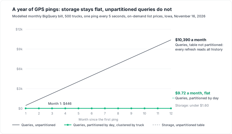
Partition by day and cluster by truck: $9.72 a month, flat
Partition the ping table on ts by day and cluster it by truck:
CREATE TABLE fleet.pings (
  truck STRING, ts TIMESTAMP, lat FLOAT64, lon FLOAT64,
  spd_kmh FLOAT64, hdg INT64, odo_km FLOAT64, ign BOOL, fuel_pct FLOAT64
)
PARTITION BY TIMESTAMP_TRUNC(ts, DAY)
CLUSTER BY truck
OPTIONS (require_partition_filter = TRUE);
The live map then reads today's partition only. Google's docs show ts = CURRENT_TIMESTAMP() as a filter that prunes partitions, so ts >= TIMESTAMP_SUB(CURRENT_TIMESTAMP(), INTERVAL 15 MINUTE) reads one day (two in the first 15 minutes after midnight UTC). In the model a refresh reads half a day on average: 1.8 million rows, 90 MB. With require_partition_filter, "every query on that table must include at least one predicate that only references the partitioning column", so a new dashboard cannot quietly scan the year.
Clustering by truck helps per-truck queries such as a customer tracking page. Google says partitions "larger than 64 MB are also likely to benefit from clustering", and a day here is 241 MB. The model gives clustering no credit, because "The cost of queries over clustered tables can only be determined after the query is run."
The strongest objection is Google's own guidance. Its list of reasons to cluster rather than partition includes "Partitioning results in a small amount of data per partition (approximately less than 10 GB)", and our BigQuery partitioning guide follows it. This fleet writes 0.24 GB a day. But the same list also includes "You don't need strict cost estimates before query execution." A live map running 25,200 times a month needs one. With month partitions and no credit for block pruning, a refresh can read half a month of pings: up to $386.76 a month for the live map alone, against $12.89. A year of day partitions is about 365, far below the "10,000 partitions" limit. For this table, day partitions are the right call.
The second objection: a live map does not belong in a warehouse. For latency that is often true. For cost, it no longer matters once the table is partitioned: $12.89 a month.
The holiday peak: a two-month bump, or a bill that stays
Consider a peak in November and December: 100 leased trucks join and every truck drives 12 hours, 1.44 times the rows. Partitioned, the peak month's queries cost $16.46 instead of $9.72, and the bump ends with the season. Unpartitioned, the 95 million extra rows join the history every later refresh reads: $795.48 more every month after the peak, for as long as the table keeps them.
Measure cost per schedule and drop what nobody reads
Tag each dashboard's queries with a job label (dashboard: live_map), then price each one from the job history, which keeps "the past 180 days":
SELECT
  (SELECT value FROM UNNEST(labels) WHERE key = 'dashboard') AS dashboard,
  COUNT(*) AS runs,
  COUNTIF(cache_hit) AS cached_runs,
  SUM(total_bytes_billed) / POW(2, 40) AS tib_billed,
  SUM(total_bytes_billed) / POW(2, 40) * 6.25 AS list_usd
FROM `region-us-central1`.INFORMATION_SCHEMA.JOBS
WHERE job_type = 'QUERY'
  AND creation_time > TIMESTAMP_SUB(CURRENT_TIMESTAMP(), INTERVAL 720 HOUR)
GROUP BY dashboard
ORDER BY list_usd DESC;
list_usd ignores the free TiB, so it ranks dashboards rather than predicting the invoice. A dashboard with zero cached_runs and a bytes-per-run figure that grows each month is reading history it does not need.
The job log cannot tell you whether anyone looked. A wall screen polling an empty dispatch office at 6 a.m. writes the same jobs as one in use. Take the viewer side from the app's access logs or the BI tool's usage data (we cover Power BI usage metrics separately), and drop any dashboard that nobody opened in 30 days. For tables that no query reads at all, the referenced_tables method in our retail data warehouse cost post applies unchanged.
Where this model stops
- List prices for Iowa, read November 16, 2026, on demand, no commitments. On editions the same refreshes cost slot-hours instead of bytes; see BigQuery on-demand vs editions.
- Every volume, schedule and screen-hour is an assumption. A refresh is modelled as reading half a day's rows; partition boundaries "are based on UTC time", so a North American fleet's evening crosses into the next partition early.
- Left out: AWS data transfer out for pings leaving AWS, ad hoc analyst queries, BI Engine, and the people who run the platform.
A live map's refresh is set in one tool, the table layout in another and the bill lands in a third. Datapace is building one map of your data estate (databases, warehouses, pipelines and what consumes them) with usage and cost attached, and agents that propose changes as pull requests your team reviews and merges. For the same fleet's stream before it reaches the warehouse, read Kinesis Data Streams pricing.
Sources
- Google Cloud, BigQuery pricing (on-demand queries, storage, long-term storage, Storage Write API, minimum bytes billed), read November 16, 2026.
- Google Cloud, Data types (logical bytes per type).
- Google Cloud: Query partitioned tables, Introduction to partitioned tables and Manage partitioned tables.
- Google Cloud, Introduction to clustered tables.
- Google Cloud, Quotas and limits (partitions per table).
- Google Cloud, INFORMATION_SCHEMA.JOBS view.
- Google Cloud, Cached query results.