
TL;DR. BigQuery cost optimization pays when it runs in order: split the bill by SKU, rank jobs by bytes billed, and check whether anyone reads what the top recurring jobs write before you tune any of them. In a worked month for a hypothetical on-demand project, the costliest mistake is tuning a job that should be stopped. An hourly scheduled query writes a table nobody has read in 90 days: tuning it would save about $1,078, stopping it saves $1,145. Counting both, as a tactics checklist does, promises $2,224 from a job worth $1,145.
BigQuery cost optimization starts with the question no tactics list asks: which line of the bill is the money, and does anyone use what it pays for? The six steps below answer it with the billing export and three INFORMATION_SCHEMA views, in the order that keeps the cheapest, safest cuts first. For the meters themselves, see BigQuery pricing: on-demand vs editions.
Every query below targets the US multi-region (region-us). Prices are US multi-region list prices from the BigQuery pricing page, read November 17, 2026: $6.25 per TiB of on-demand analysis after a free first TiB each month, and $0.02 per GiB-month of active logical storage. The worked month is a hypothetical project, not a measurement, and the queries follow Google's documentation of that date; none was tested on a live account here.
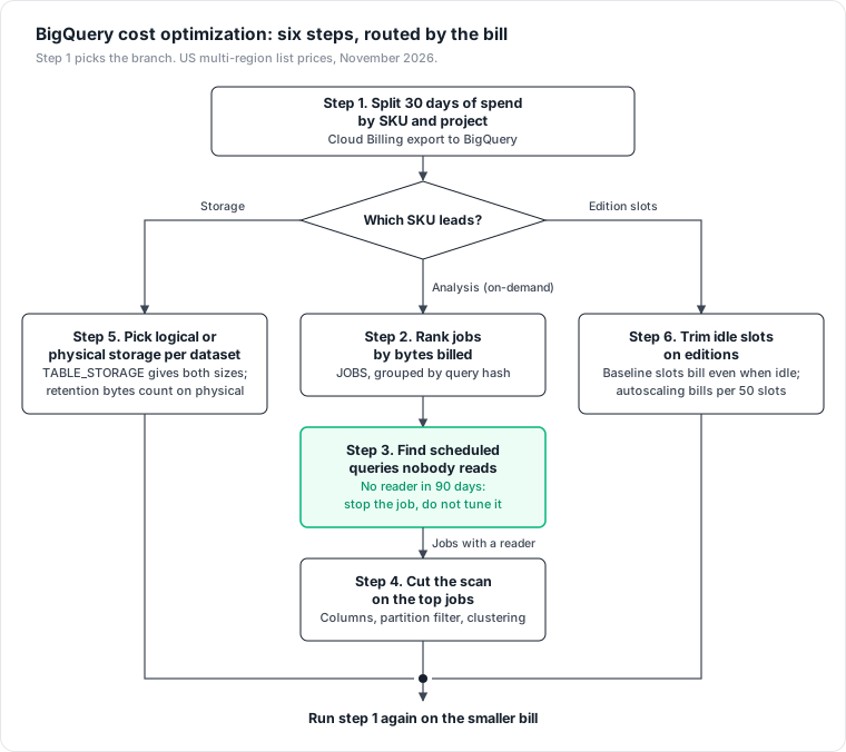
Step 1: split 30 days of BigQuery spend by SKU and project
The Cloud Billing standard export writes your costs to a table named gcp_billing_export_v1_<BILLING_ACCOUNT_ID>, with SKU, project and labels on each row and usage in hourly windows. If you enable it for the first time on a US or EU multi-region dataset, Google backfills data "from the start of the previous month", which is enough for a 30-day split.
-- Step 1: BigQuery spend by SKU and project, last 30 days
SELECT
  project.id                      AS project_id,
  sku.description                 AS sku,
  ROUND(SUM(cost), 2)             AS cost,
  ROUND(SUM(IFNULL((SELECT SUM(c.amount) FROM UNNEST(credits) c), 0)), 2) AS credits,
  ROUND(100 * SUM(cost) / SUM(SUM(cost)) OVER (), 1) AS pct_of_cost
FROM `billing-admin.billing_export.gcp_billing_export_v1_XXXXXX_XXXXXX_XXXXXX`
WHERE service.description LIKE 'BigQuery%'
  AND usage_start_time >= TIMESTAMP_SUB(CURRENT_TIMESTAMP(), INTERVAL 30 DAY)
GROUP BY project_id, sku
ORDER BY cost DESC;
The top SKU picks your branch. Google says on-demand pricing "is referred to as analysis pricing" on its SKU list, so an "Analysis" row on top sends you to step 2. Storage rows on top send you to step 5, edition slot rows to step 6. cost includes negotiated discounts; credits sit in their own column so they do not hide a growing line.
Step 2: rank jobs by bytes billed
-- Step 2: the 25 query shapes that bill the most bytes, last 30 days
DECLARE usd_per_tib FLOAT64 DEFAULT 6.25;  -- US multi-region on-demand, Nov 17, 2026

SELECT
  query_info.query_hashes.normalized_literals                   AS query_hash,
  ANY_VALUE(destination_table.dataset_id || '.' || destination_table.table_id) AS writes_to,
  ANY_VALUE(user_email)                                         AS run_by,
  COUNT(*)                                                      AS runs,
  ROUND(SUM(total_bytes_billed) / POW(1024, 4), 2)              AS tib_billed,
  ROUND(SUM(total_bytes_billed) / POW(1024, 4) * usd_per_tib, 2) AS usd_at_list,
  ANY_VALUE(LEFT(query, 160))                                   AS sample
FROM `region-us`.INFORMATION_SCHEMA.JOBS
WHERE creation_time >= TIMESTAMP_SUB(CURRENT_TIMESTAMP(), INTERVAL 30 DAY)
  AND job_type = 'QUERY'
  AND (statement_type IS NULL OR statement_type != 'SCRIPT')
GROUP BY query_hash
ORDER BY tib_billed DESC
LIMIT 25;
The JOBS view keeps 180 days of history and needs a region qualifier. The hash "ignores comments, parameter values, UDFs, and literals", so an hourly job with a new timestamp in each run collapses into one row with runs at about 720. Failed runs and cache hits have no hash and share one NULL row. Multi-statement parents (SCRIPT) are excluded because their children carry the same bytes. The dollar column ignores the free TiB, which is per billing account.
A recurring job near the top is your first suspect, and the next step checks it before anyone tunes it. One limit: JOBS covers one project. If your readers run queries from other projects, use the organization-wide JOBS_BY_ORGANIZATION view.
Step 3: find scheduled queries nobody reads
A scheduled query, a dbt model or an Airflow task bills its bytes every run whether or not anyone opens the result. JOBS records both sides: destination_table for what a job writes, and referenced_tables for what it reads.
-- Step 3: tables written in the last 90 days that no other query read
WITH writes AS (
  SELECT destination_table.project_id AS project_id,
         destination_table.dataset_id AS dataset_id,
         destination_table.table_id   AS table_id,
         COUNT(*)                     AS write_jobs,
         ROUND(SUM(total_bytes_billed) / POW(1024, 4) * 6.25, 2) AS write_usd_at_list
  FROM `region-us`.INFORMATION_SCHEMA.JOBS
  WHERE creation_time >= TIMESTAMP_SUB(CURRENT_TIMESTAMP(), INTERVAL 90 DAY)
    AND job_type = 'QUERY'
    AND (statement_type IS NULL OR statement_type != 'SCRIPT')
    AND destination_table.table_id IS NOT NULL
    AND NOT STARTS_WITH(destination_table.dataset_id, '_')  -- skip anonymous result tables
  GROUP BY 1, 2, 3
),
reads AS (
  SELECT DISTINCT t.project_id, t.dataset_id, t.table_id
  FROM `region-us`.INFORMATION_SCHEMA.JOBS j, UNNEST(j.referenced_tables) t
  WHERE j.creation_time >= TIMESTAMP_SUB(CURRENT_TIMESTAMP(), INTERVAL 90 DAY)
    AND j.job_type = 'QUERY'
    AND NOT (IFNULL(j.destination_table.dataset_id, '') = t.dataset_id
             AND IFNULL(j.destination_table.table_id, '') = t.table_id)  -- a job reading its own target is not a reader
)
SELECT w.*
FROM writes w
LEFT JOIN reads r USING (project_id, dataset_id, table_id)
WHERE r.table_id IS NULL
ORDER BY write_usd_at_list DESC;
Every row is a table that costs money to produce and that no query read in 90 days. Stop its schedule, keep the table for a few weeks in case someone asks, then drop it. Do this before step 4: tuning a job nobody reads makes it cheaper and keeps it running forever.
The check misses readers that never run a query. Google documents referenced_tables as "only populated for query jobs that are not cache hits". A table read only through the Storage Read API, which Google lists as its own access path beside tabledata.list and extract jobs, or exported to Cloud Storage leaves no query read. For MERGE or INSERT jobs, confirm on one known job that destination_table holds the target before trusting an empty result. Treat each row as a question for the owner, the same rule as in Snowflake access history.
Step 4: cut the scan on the top jobs
For the jobs that keep a reader, on-demand bills bytes, so fewer bytes read is the saving. Google bills "the data processed in the columns you select, even if you set an explicit LIMIT on the results."
- Name the columns.
SELECT *bills every column of every row scanned. A dashboard that needs four narrow columns pays for the wide ones too. - Filter on the partition column. Only queries that filter on it skip partitions; the BigQuery partitioning post covers when a table should be partitioned and what the rewrite costs.
- Cluster on the filter and join columns. Clustered queries "scan only the relevant blocks", but Google warns you "don't receive an accurate cost estimate before execution", so measure after.
- Precompute repeated aggregates. Google positions materialized views for "repetitive, expensive queries over large datasets"; BigQuery keeps them up to date as base tables change.
On editions none of these shows up as bytes on the invoice: the saving is slot time, which the total_slot_ms column reports per job.
Step 5: pick logical or physical storage per dataset
Storage is billed per dataset on logical (uncompressed) or physical (compressed) bytes. In the US multi-region, logical costs $0.02 per GiB-month active and $0.01 long-term; physical costs $0.04 and $0.02. Data moves to the long-term rate after "90 consecutive days" without modification, per partition. A CREATE OR REPLACE TABLE, a load or any write into the table resets the clock.
-- Step 5: monthly storage cost per dataset under each billing model (US multi-region)
SELECT
  table_schema AS dataset,
  ROUND(SUM(IF(deleted = FALSE, active_logical_bytes, 0))    / POW(1024, 3) * 0.02
      + SUM(IF(deleted = FALSE, long_term_logical_bytes, 0)) / POW(1024, 3) * 0.01, 2) AS logical_usd,
  ROUND((SUM(active_physical_bytes) + SUM(fail_safe_physical_bytes)) / POW(1024, 3) * 0.04
      + SUM(long_term_physical_bytes) / POW(1024, 3) * 0.02, 2)                      AS physical_usd,
  ROUND(SUM(time_travel_physical_bytes + fail_safe_physical_bytes) / POW(1024, 3), 1) AS retention_gib
FROM `region-us`.INFORMATION_SCHEMA.TABLE_STORAGE
WHERE table_type = 'BASE TABLE'
GROUP BY dataset
ORDER BY logical_usd DESC;
The formulas follow Google's own forecast in the TABLE_STORAGE docs, where active_physical_bytes already includes time travel bytes. Under physical billing, time travel and fail-safe bytes are billed at active rates; under logical billing they are included. So an append-only dataset that compresses well is the candidate, and a dataset of tables rewritten every hour is not. A switch takes 24 hours to apply and blocks another switch for 14 days, and the time travel window can be cut from the default seven days to two.
Step 6: trim idle slots on editions
If edition slots lead step 1, the waste sits in reserved capacity. Google states that baseline slots "will always be allocated to the reservation, and you will always be charged for them", and that autoscaling charges "for the number of scaled slots, not the number of slots used", in multiples of 50 with a one-minute minimum by default.
-- Step 6: what each reservation holds, run in the reservation admin project
SELECT reservation_name, edition,
       slot_capacity       AS baseline_slots,
       autoscale.max_slots AS autoscale_max_slots,
       ignore_idle_slots
FROM `region-us`.INFORMATION_SCHEMA.RESERVATIONS;
A baseline is a fixed monthly bill. 100 baseline slots on Enterprise pay-as-you-go at $0.06 per slot-hour cost 100 × 730 hours × $0.06 = $4,380 in an average month whether queries run or not. Compare each baseline with the slots your jobs use per second from JOBS_TIMELINE; the utilization query in the on-demand vs editions post gives that number. Then lower the baseline toward what never idles and cap autoscale.max_slots.
A worked month: one job to stop, one to tune
Consider a hypothetical on-demand project in the US multi-region, priced at list:
| Line | Monthly volume | Cost |
|---|---|---|
A. Hourly scheduled query overwriting sessions_hourly, no reader in 90 days | 0.25 TiB × 720 runs = 180 TiB | $1,125.00 |
B. Dashboard, SELECT * on events, 300 runs | 0.80 TiB × 300 = 240 TiB | $1,500.00 |
C. Nightly CREATE OR REPLACE of orders_wide, read daily | 2 TiB × 30 = 60 TiB | $375.00 |
| D. Ad hoc analysis | 75 TiB | $468.75 |
| Analysis, less the free TiB | 555 − 1 = 554 TiB | $3,462.50 |
Storage, logical: 8 TiB active and 22 TiB long-term in events, 4 TiB always active in the marts (1 TiB sessions_hourly, 3 TiB orders_wide) | 12,288 GiB × $0.02 + 22,528 GiB × $0.01 | $471.04 |
| Total | $3,933.54 |
The cuts, in step order:
| Step | Change | Monthly saving |
|---|---|---|
| 3 | Stop job A and drop its 1 TiB table: $1,125.00 + 1,024 GiB × $0.02 | $1,145.48 |
| 4 | Dashboard B names the columns holding 20% of the bytes: 240 TiB to 48 TiB | $1,200.00 |
| 5 | events to physical billing, assuming 4 to 1 compression and few time travel bytes because it is append-only: $389.12 logical to $194.56 physical | $194.56 |
| Total | $2,540.04, 64.6% of the bill |
The order matters most on job A. Started from a tactics list, step 4 reaches A, the second-largest job, and tunes it. If A rescans the last 24 hours of an hourly-partitioned input every hour, making it incremental (read only the newest hour and merge it into sessions_hourly) saves $1,125 × 23/24 = $1,078.13 and leaves it running. Sized separately, the two levers promise $2,223.61 from a job that can give $1,145.48. Job C stays: it has a reader.
The model's limits: real bills mix on-demand and edition projects, the 20% column share and 4 to 1 compression are assumptions to replace with your own numbers, and the model ignores cache hits, which bill no bytes.
Apply the cuts reversible first
The strongest objection to this order is that stopping jobs takes owners, meetings and time, while a byte limit takes minutes. That is right for the first week. Set guards first, then do the steps:
- Maximum bytes billed on scheduled jobs and BI service accounts: a query over the limit "fails without incurring a charge." On clustered tables the estimate is an upper bound, so a query can fail even when its actual bytes would stay under the limit.
- A custom daily quota that applies to each user and service account (
QueryUsagePerUserPerDay) and one per project (QueryUsagePerDay, 200 TiB by default). Quotas apply only to on-demand, reset at midnight Pacific, and Google calls them approximate. - Stop unread jobs (step 3), which you can restart if an owner objects.
- Rewrite queries and tables (steps 4 and 5) last, since they take engineering time and a test.
Guards cap the damage; they do not find the job nobody reads. BigQuery is one line of the platform bill, and the cloud waste in data infrastructure post covers unread data and idle capacity across the rest.
Datapace is building one map of your data estate with usage and cost attached, and agents that propose changes as pull requests your team reviews and merges. For the same sequence on another platform, read Databricks cost optimization, or book a call.